Getting the Data You Want
Oracle Discoverer Tutorial

	Getting the Data You Want	Oracle Discoverer Tutorial

Tip: Print this page.

The total estimated time you need to complete lesson 2 is 30 minutes.

Overview of Lesson 2

In Lesson 2, you will choose layout defaults for new Workbooks that you create using the Workbook Wizard. After you create a new Workbook, you will organize Items and Page Items on your table Worksheet. You will duplicate your table Worksheet as a crosstab Worksheet. Then, you will reduce the amount of data in your Worksheet by creating conditions and parameters. Finally, you will add new Items to your new Workbook.

Selecting layout defaults for your Worksheets

Before you create a new Workbook, you can decide how you want the data in your Workbook to look. For example, you can choose font size, background color, and text alignment. The choices you make become the default settings for all new Workbooks. You can later change your mind and change the default settings. However, default settings affect only new Workbooks from that time forward. They do not change the layout of Workbooks that you already created or that were created by someone else.

Launch Discoverer and connect to the Video Store database. Did you forget how? Click here for a Hint.
The Workbook Wizard appears, which guides you through the steps necessary for getting the data you want from the database. For now, click the Cancel button. The Workbook Wizard closes.
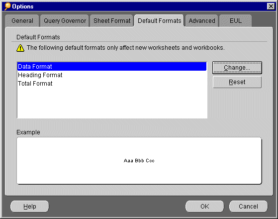
From the menu bar at the top of the Discoverer window, choose Tools | Options. The Options dialog appears with the General tab active. You use the Options dialog to choose default settings for using Discoverer. Options customize Discoverer to your work preferences.
Click the Default Formats tab.
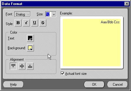
If it is not already highlighted, click Data Format, and then click the Change... button. The Data Format dialog appears, which you use to choose font styles for data in new Worksheets.
On the right side of the Data Format dialog, you see an example of the current font settings. On the left side of the Data Format dialog, click the B button and notice how the example text changes to bold. The example changes every time you change text features. Change some of the font settings and notice how the example changes: choose a font size that you like from the Size drop-down list, choose a color for your text and a background color in the Color group box, and choose the vertical alignment you like.
When you are finished, click OK. The Data Format dialog closes.
If you want, change the default formats for headings and totals also. The Heading Format selection affects row and column headings, and the Total Format selection affects how totals are displayed; for example, if you want your grand totals for profits and sales to stand out, make total format bold and a larger size than data format.
Click OK to close the Default Formats dialog.

QUESTION: Do your layout options affect Workbooks created by other people, even if you open them on your own computer? Answer.
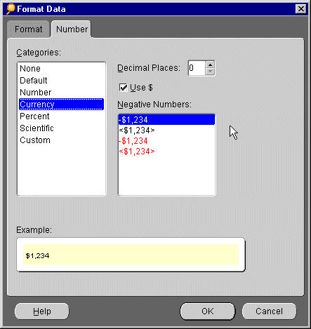
NOTE: You can make changes to the layout of your Workbooks later, using the Format tab on the Edit Worksheet dialog. For example, you may want to change the format of your currency.

Creating a new Workbook

For the moment, we will put aside the tutorial Workbook Video Stores Analysis, and create our own Workbook.

Before you can get the data you want, you must create a new Workbook using the Workbook Wizard. With the Workbook Wizard, you select Items from the video store database. The Items you choose determine the data you get. You must also decide how you want to display the data you get from the database.

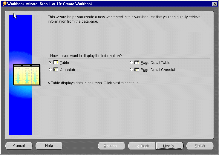
From the Discoverer menu, choose File | New. The Workbook Wizard appears.
The Workbook Wizard asks you how you want to display the data that you will get from the database. Discoverer gives you four ways to display data:
- Table
- Page-Detail Table
- Crosstab
- Page-Detail Crosstab
The simplest way to display your data is in a table. A table displays data in columns with column headings. Click Table and then click the Next button.
The next page of the Workbook Wizard asks you to select Items from the database. By selecting Items, you decide which data you want to get and analyze in your table. On the left side of the Workbook Wizard, click the arrow below the word Available. From the drop-down list, choose Video Store Tutorial. The choices you see in the drop-down list are different parts of your company's database that your Discoverer Administrator has organized for you - these are called Business Areas.
Business Areas contain data specific to your area of interest; for example, an Accounts Payable Business Area, a Sales Business Area, and an Operations Business Area. Your Discoverer Administrator creates Business Areas for the whole company and grants access and other privileges to each Business Area.
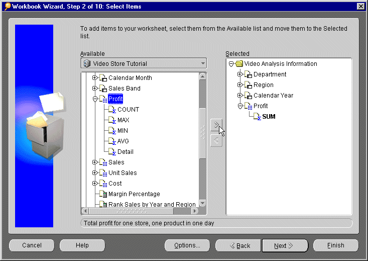
In the Available group box, click the [+] next to Video Analysis Information. The [+] becomes a [–] and Video Analysis Information expands to show a list of all Items that you can get from the video store database. For example, the first Item in the list, Department, contains data about the departments at the video stores.
Click the word Department and add it to the Selected group box.
To add an Item, you can either drag-and-drop it to the Selected group box, or you can use the left arrow and right arrow buttons.
In the Available group box, click the [+] next to the Profit Item so that Profit expands to show a list of additional Items.
Add Region and Calendar Year and to the selected list.
Add Profit SUM to the Selected group box.
For numerical data like sales, costs, and profits, Discoverer provides you with a choice of aggregations, or summaries. For example, if you want to know the total profit for a particular region, choose SUM. If you want to know the average profit for the same region, choose AVG.

You should now have the following Items in your selected list:

Department

Region

Calendar Year

Profit SUM

QUESTION: Which aggregate moved: SUM, COUNT, MAX, MIN, AVG, or Detail? Answer.
Click Next to display the Format page. In our case will accept the default Format settings.
Click Next to display the Table Layout page.
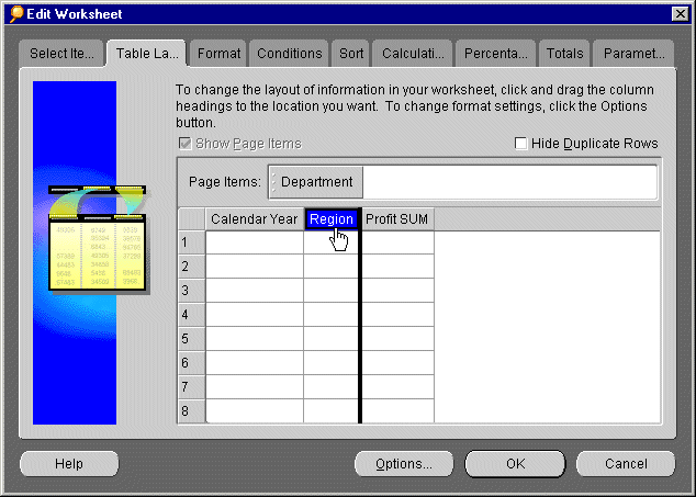
You can see that Department is in the Page Items area. Region, Calendar Year, and Profit SUM are in the rest of the Worksheet.
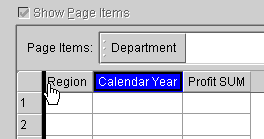
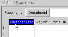
To re-order the Items, click the Calendar Year Item and drag it to the left of the Region Item. A black bar between the columns shows you where the Item will be positioned.
Click next to display the Conditions page.
Click the check box next to Department is Video Rental or Video Sale. This will restrict our data to only the Video Rental and Video Sale Departments.
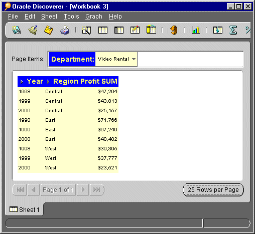
Click the Finish button. A new Worksheet, called Sheet 1, appears. Sheet 1 contains the data for the Items you selected. Notice the column headings; they match the Items that you chose in the Workbook Wizard.

Saving your Workbooks

Discoverer saves your Workbooks in your company's database. Your Discoverer Administrator must grant you the privilege to save Workbooks in the database. If you try the procedure below and find that you cannot save your Workbook, it is likely that your Discoverer Administrator has not granted you this privilege. If you cannot save your work, stay connected to the video store database instead for the duration of this lesson. You will occasionally see a warning that asks if you want to stay connected. If so, click Yes.

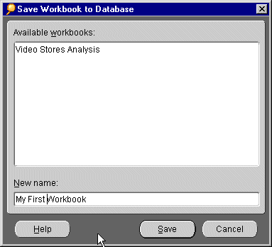
From the Discoverer menu bar, choose File | Save As. The Save Workbook to Database dialog appears.
In the text field under the label, New name, type a name for your Workbook; for example, My First Workbook.
Click the Save button.

QUESTION: Where will you find the name of your Workbook on the Workbook itself? Answer.

Working with the Worksheet

The data you got from the database contains columns of information. The rows are disorganized and not yet useful for any meaningful analysis. In Lesson 3 you will learn to use Discoverer's most powerful features: its data analysis tools. After you organize your data for analysis, you will add more Items to the table.

One technique you can use to organize your data is to create Page Items. For example, Sheet 1 contains data for two departments at the video stores: Video Rental and Video Sale. With Page Items, you can organize your data so that you get a separate page for each department.

However, suppose you want to see your data organized by region instead of department. To create a separate page for each region, you must move region to the Page Items area.

From the menu, choose Sheet | Edit Sheet. The Edit Worksheet dialog appears. Notice that the Edit Worksheet dialog looks like the Workbook Wizard. Discoverer provides you with both methods for getting the data you want, analyzing your data, and sharing your results with others. However, you use the Edit Worksheet dialog after you have already chosen some initial data with the Workbook Wizard.
Click the Table Layout tab. With the Table Layout tab, you create Page Items and re-arrange the columns on your Worksheet. The Table Layout tab does not affect the data itself; it just re-organizes the data.

Notice the checkmark in the box next to the words Show Page Items. This check box allows you to create Page Items. In this example, the box is already checked and the Department Item appears in the Page Items text field.
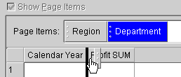
Click the Region and drag it into the Page Items text field next to Department.
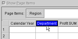
Click the Item, Department, and drag it down into the main body of the table. Notice that a black line appears that indicates the new position of the Item's column. Drag-and-drop Department so that it is positioned between the Calendar Year and Profit SUM Items.
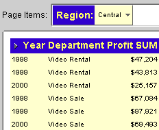
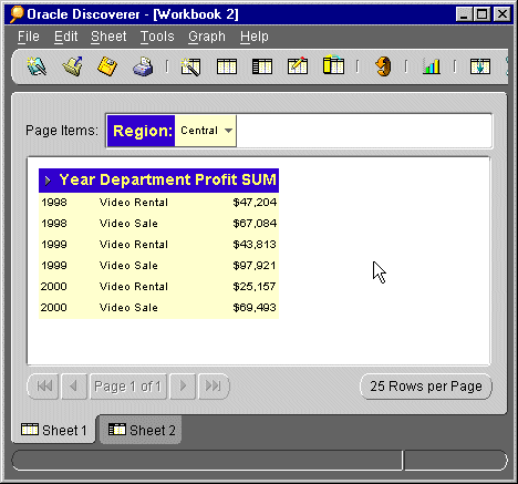
Click OK. The Worksheet appears, re-organized by Region. Notice that Page Items: Region appears at the top of the Workbook window. The Department Item is now displayed between the Year and Profit SUM columns. For which region are you viewing data? Click the word Region and choose another region from the drop-down list. Notice how the data changes.
Save your work. Hint.

Changing from a Table layout to a Crosstab layout

Another way to organize your data for analysis is to duplicate your table as a crosstab. A crosstab relates two sets of data and then summarizes their interrelationship in terms of a third set of data. For example, a typical crosstab for the video stores shows the monthly profit for each region, organized by department. In other words, there are three sets of data: total sales, region, and department. 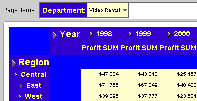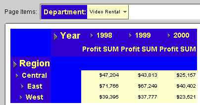By duplicating your table as a crosstab, Discoverer calculates a subtotal of the profit for each region, as shown below.

In the screen shot above, notice that you now have new data, the subtotal of profit for each Region for each Year. Notice also that the Regions appear on the left side as row headings. In addition to columns, crosstabs also have rows.

From the menu, choose Sheet | Duplicate as Crosstab.

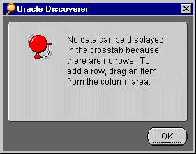
A warning appears to let you know that you must have rows defined in a crosstab. Rows on Crosstabs are side axis items. Click OK.
The Edit Worksheet dialog appears again, open to the Crosstab Layout tab.
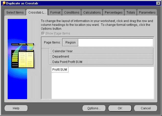
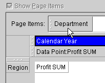
Notice in the Crosstab Layout screenshot below that there are no side axis Items on the left hand side. The three Items Calendar Year, Department, and Data Point:Profit SUM, all appear on the top axis.

The Crosstab Layout tab looks very similar to the Table Layout tab that you have already seen.

Notice that the column heading, Department, and a new one called Data Point:Profit SUM appear by themselves. Calendar Year, Department and Data Points are top axis Items because they appear on top of other Items. When you create a crosstab, you must choose which column headings become the top and side axis Items. You can rearrange axis Items whenever you want from the Edit Sheet dialog.
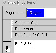
Drag the Region Item from the Page Items are to the side axis area.
Drag the Department Item to the Page Items area.
Click OK. If you are unclear about axis Items, look at the new Worksheet. Notice that the crosstab is organized by Region on the left axis Item. And notice that Department is the top axis Item.
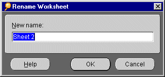
If you would like to rename your new Crosstab Worksheet, double click the Sheet 2 tab at the bottom of the Worksheet.
Type in a new name and click OK.

Filtering data with conditions

Some video stores show larger profits than others. What factors cause some stores to earn more profit than others? If you are getting data from a very large database, the amount of data you get could be so large that you would have difficulty finding the answer to that question. So if you are interested in analyzing only the stores with the highest profits, how could you reduce the amount of data you get from the database?

Discoverer provides you with a tool called conditions that reduces the amount of data you get from the database. Conditions filter data to exclude some information so that the data is more manageable. For example, if you want to analyze stores with the highest profits, you could create a condition that says "Show me regions with annual profit great than 50,000 dollars".

To return to the Tabular Worksheet, click Sheet 1 tab at the bottom of the Workbook.
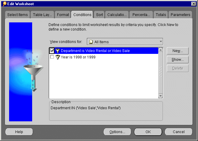
From the menu, choose Tools | Conditions. The Edit Worksheet dialog appears, open to the Conditions tab.
Notice that two conditions already exist. They were created for you by the Discoverer Administrator at your company. Some conditions have check marks next to them and some do not. The conditions with checkmarks next to them are active, or turned on, in this Worksheet.
Select the check box next to 'Department is Video Rental or Video Sale' to restrict your Worksheet to profits in these Departments.
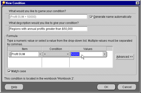
You are going to create a new condition. Click New. You will create a new condition to limit the data to Regions with annual profit over 50,000 dollars.
If the Generate name automatically is not selected, click this check box. Discoverer will create a condition name for you.
In the text field under What description would you like to give your condition? type, Regions with annual profits greater than $50,000. This description appears in the Conditions tab. If the name is unclear, the description you write helps other users understand the purpose of your condition.
Look at the Formula group box. This is where you create the condition's formula. Discoverer displays any data that equals the formula and ignores any data that doesn't equal the formula. In this example, Discoverer displays any data about regions with profits greater than 50,000 dollars and ignores all other data. From the left-most drop-down list, select Video Analysis Information.Profit SUM. From the middle drop-down list, select the "greater than" symbol [>]. In the right-most text field, type 50000.
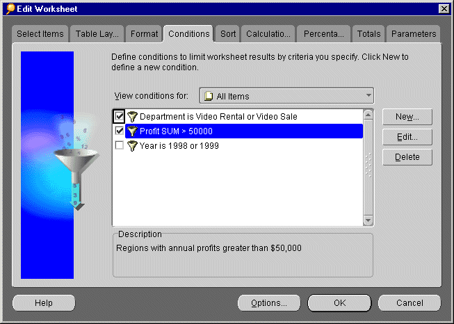
Click OK. Discoverer returns you to the Conditions tab.
Notice the name of your new condition: Profit SUM > 50000. This is the condition name that Discoverer generated automatically for you. You can see the description that you typed in below: Regions with annual profits greater than $50,000. The checkmark next to the name means that the new condition is turned on. If you want to turn off the condition, uncheck the checkbox.
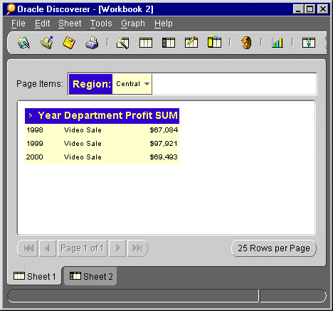
Click OK. Discoverer sends a new query to the database and shows you the new results in the Worksheet. Notice that you now have less data. Only regions with annual profits greater than 50,000 dollars are shown.

As you can see, only for the Video Sale Department in the Central Region did profits exceed $50,000.

NOTE: Another way to highlight data is to use Discoverer Exceptions. Here, the data in the Worksheet is not restricted, but values that match a specified figure are highlighted. Refer to the Discoverer 4i Plus User's Guide for information about using Exceptions.
When you have finished working with the Worksheet, remember to turn off you Condition Profit SUM > 50000. Choose Tools\Conditions, then uncheck the Profit SUM > 50000 Condition check box.

Creating parameters for other users

Sometimes you may open this Workbook and want to see data about the year 2000, and sometimes you may want to see data about the year 1999. Or perhaps you want to share this Workbook with another person, and you do not know what Year they want to see. Discoverer gives you another tool, parameters, which gives you and other users a choice of filters when a Workbook opens.

You will create a new parameter that asks you which Year you want to look at. Every time you or another person opens this Workbook, Discoverer will ask you to which Year you want to look at.

Make sure that you have turned off the Condition Profit SUM > 50000, (see step 12 in the previous task).
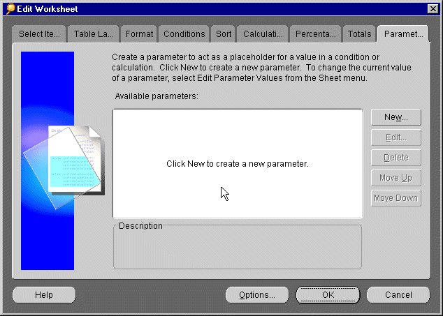
From the menu, choose Tools | Parameters. The Edit Worksheet dialog appears, open to the Parameters tab. The Parameters tab lists all the parameters that already exist for this Workbook. A checkmark next to a parameter indicates that it is turned on.
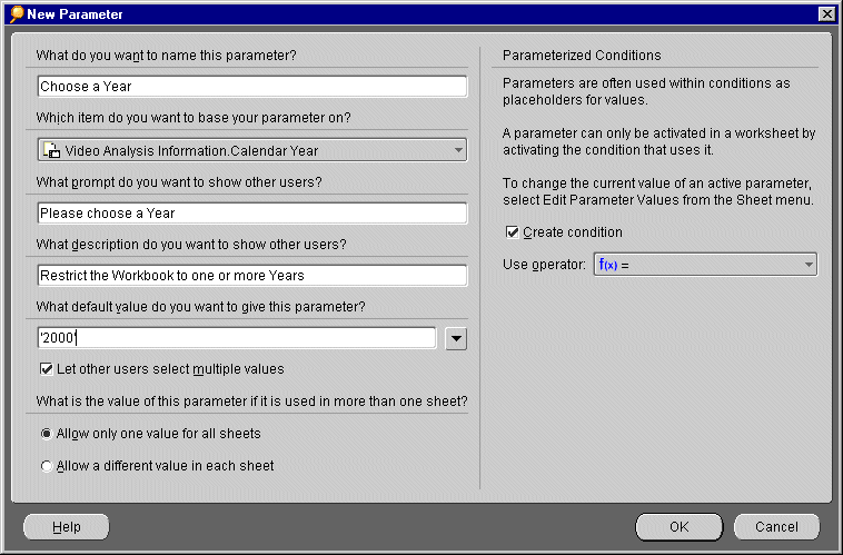
Click New to create a new parameter. The New Parameter dialog appears.
In the text field under What do you want to name this parameter?, type Choose a Year.
From the drop-down list under Which Item do you want to base this parameter on?, select Video Analysis Information. Calendar Year.
In the text field under What prompt do you want to show other users?, type Please choose a Year. Every time this Workbook opens, you or other users will see this prompt.
In the text field under What description do you want to show other users?, type Restrict the Workbook to one or more Years. Every time this Workbook opens, you or others will see this description. If the prompt or name is unclear, the description you write helps other users understand the purpose of your parameter.
Click the drop-down list under the question What default value do you want to give this parameter? and click 2000. Every time this Workbook opens, 2000 will be the default choice that users see when asked to choose a Year.
Put a checkmark in the box next to Let users select multiple values. If you or another user wants to see data for both 1999 and 2000, ticking this checkbox allows you to select more than one Year at a time.
Leave the default value for Allow only one value for all sheets selected. The Parameter will apply to all Worksheets in the Workbook.
Leave the default value for Create condition option selected. A new Condition will be created, which will allow us to turn this Parameter on and off.
Click OK. Discoverer returns you to the Parameters dialog.
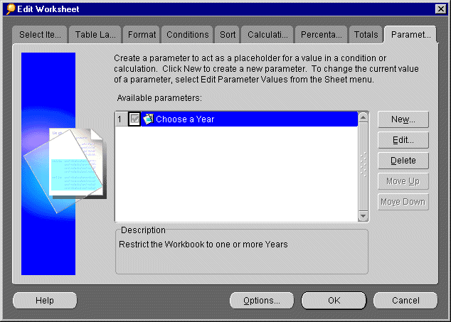
Notice that your new parameter, called Choose a Year, appears with a checkmark next to it. Look at the Description box at the bottom. The description you wrote, Restrict the Workbook to one or more Years, appears also.
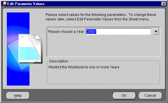
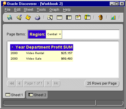
Click OK. The Edit Parameter Values dialog appears and asks you to choose which Year you want.
Accept the default value '2000' from the drop-down menu and click OK. Discoverer sends a new query to the database and displays the Worksheet. Only data for the year 2000 appears in the Worksheet.

Notice that only data for the Year 2000 is displayed on your Worksheet. You are also restricting your worksheet to data for the Central Region using the Region Page Item.
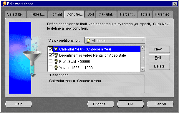
Because you checked the Create condition option when you created the parameter, you can turn this parameter value off and on using the Conditions dialog. Choose Tools\Conditions and uncheck the Calendar Year = :Choose a Year condition to turn this value off.

What is the difference between a condition and a parameter? Answer.

How do you turn conditions on and off? Answer.

Adding more Items to the Worksheet

Now that you have begun to organize your data for analysis, you realize that you need more information in your table. You know the Profit for each region, but you would also like to see Sales.

Return to the Tabular Worksheet by clicking the Sheet 1 tab at the bottom of the Worksheet.
From the menu, choose Sheet | Edit Sheet. Once again, the Edit Worksheet dialog appears.
If it is not already clicked, click the Select Items tab. Once again, you see the Available group box and the Selected group box. Click the [+] next to Video Analysis Information, which expands to show you a list of additional Items. From the list of Items, move Sales SUM to the Selected group box.
Click the Table Layout tab. Drag-and-drop the Items so that they are organized in the following order: Calendar Year, Department, Profit SUM, and Sales SUM.
Click OK.

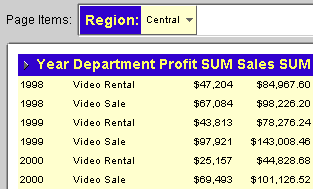
Your Worksheet now contains the new Item Sales SUM. You can now analyze how Sales relate to Profit figures.

Summary of Lesson 2

In lesson 2 you got the data you want from the database and made choices about how the data appears. By selecting layout defaults, you customized the way all new Workbooks look after you create them. Layout defaults do not affect Workbooks created by other people or Workbooks that you created before you changed the defaults, only new Workbooks created after you change defaults.

You used the Workbook Wizard to create a new Workbook by selecting Items that you want to see in your Worksheet. Later, you went back to the Workbook Wizard to add more Items to your Worksheet. You can add or delete Items from Worksheets at any time using the Workbook Wizard. After saving your Workbook in the database, you arranged Items into Page Items and axis Items to make analysis easier. You then created conditions that reduce data in your Worksheets to make them more manageable. You also created parameters, which give you the choice of filters when the Workbook opens.

Return to Tutorial Home Page

Answers and Definitions

Do your layout options affect Workbooks created by other people, even if you open them on your own computer?

No, your layout options only affect the Workbooks you create after the time you choose your options. If you change your layout options, only new Workbooks are affected. Old Workbooks or Workbooks created by other people retain the layout options that were in effect at the time they were created.

Which aggregate moved: SUM, COUNT, MAX, MIN, AVG, or Detail?

SUM moved. In this example, Discoverer defaults to SUM for aggregations. Your Discoverer Administrator decides which type of aggregation to use as the default.

Where will you find the name of your Workbook on the Workbook itself?

The Workbook's name appears at the top of the Workbook, in brackets. For example, [Video Stores Analysis].

What is the difference between a condition and a parameter?

A condition filters data in the same way every time the Workbook opens. Parameters offer you and other users a choice of filters to use.

How do you turn conditions on and off?

From the Tools menu, choose Conditions. In the Conditions dialog, you see a list of conditions that already exist. A checkmark next to the name indicates that the condition is turned on. By removing the checkmark, you turn the condition off.

Items. An Item is a name for a specific set of data in the database; for example, if you want to see all departments in the database, you select the Department Item. In a Worksheet, Items appear as column and row headings.